- 개요
folium에서는 Choropleth이나 Polygon을 이용하여 지도에 선(contour)을 그리고, 특정 색상(shading)으로 칠할 수 있습니다.
하지만 folium에서 이를 쓰려면 각 polygon의 위도, 경도값을 알아야 합니다.
만약 특정 지역마다 온도값을 표현한다면 각 지역의 polygon 정보를 구한 뒤 folium을 사용해서 온도의 공간 분포를 시각화해도 됩니다.
문제는 각 위도, 경도 정보를 격자형태로 가진 온도를 시각화할 때 생깁니다.
Matplotlib 라이브러리로 위도, 경도의 차원인 온도를 그린다고 쳐봅시다.
Matplotlib에서 contour나 contourf에 위도, 경도, 온도 값을 적당히 넣어주고 plot.show()를 치면 알아서 화면에 선도 그려주고 색도 칠해줍니다.
여기서 contour, contourf는 위도, 경도, 온도와 contour level 정보에 따라 선에 대한 polygon 정보를 만들어줍니다.
folium은 입력값에 따라 polygon의 좌표를 만들어주는 기능이 없기 때문에 matplotlib의 기능을 이용하면 folium 지도 위에 온도 공간 분포를 시각화 할 수 있습니다.
- Matplotlib에서 선에 대한 polygon 정보 얻기
cs = plt.contourf(lat2d, lon2d, plot_var.T)를 선언하면 cs.allseg, cs.allkinds 변수를 얻을 수 있습니다.
cs.allsegs에는 위도, 경도값, cs.allkinds에는 선의 시작과 끝에 대한 정보가 있습니다.
참고로 cs.allkinds를 print로 확인하면 숫자 1, 2, 79가 있습니다.
1은 선의 시작, 2는 선이 이어지는 것, 79는 선의 종료를 의미합니다.
그리고 matplotlib에서 아무 옵션을 설정하지 않고 contour를 그리면 기본으로 8개의 contour level을 설정하기 때문에 cs.allsegs, cs.allkinds의 길이는 8입니다.
import matplotlib.pyplot as plt
"""
plot_var 변수는 위도, 경도 차원이고 온도값을 가지고 있습니다.
plt.contourf은 원래 경도, 위도, 변수의 순서로 인수를 받아야 합니다.
하지만 이번 예제에서 folium의 polygon 좌표값은 위도, 경도 순이라서
위도, 경도 순으로 값을 넣어줍니다.
위도, 경도의 순서가 바뀌어서 변수(여기서는 plot_var)를 transpose(뒤에 .T) 합니다.
"""
cs = plt.contourf(lat2d, lon2d, plot_var.T)

allsegs = cs.allsegs # 선의 위도, 경도값이 들어있음
allkinds = cs.allkinds # 선의 시작과 끝에 대한 정보가 들어있음

print(cs.allsegs)
""" 결과
[[array([[ 32.41001089, 120.20952599],
       [ 32.41132089, 120.23093599],
       [ 32.41263089, 120.25235479],
       ...,
       [ 32.3751058 , 120.20005062],
       [ 32.3932658 , 120.19850062],...
"""
print(cs.allkinds)
""" 결과
[[array([ 1,  2,  2,  2,  2,  2,  2,  2,  2,  2,  2,  2,  2,  2,  2,  2,  2,
        2,  2,  2,  2,  2,  2,  2,  2,  2,  2,  2,  2,  2,  2,  2,  2,  2,
...
2,  2,  2,  2,  2,  2,  2,  2,  2,  2,  2,  2,  2,  2,  2,  2,  2,
        2,  2,  2,  2,  2,  2,  2,  2,  2,  2,  2,  2,  2,  2,  2,  2,  2,
        2,  2,  2,  2,  2,  2, 79], dtype=uint8)]]
"""
- folium에 쓰기 적합하도록 cs.allsegs, cs.allkinds를 전처리하는 함수 작성
cs.allkinds에서 선의 시작과 끝인 인덱스를 찾고 이에 해당하는 위도와 경도값을 리스트로 반환하는 함수입니다.
stackoverflow의 문서를 참고했습니다.
참고문헌: https://stackoverflow.com/questions/65634602/plotting-contours-with-ipyleaflet
import numpy as np

def split_contours(segs, kinds=None):
    if kinds is None:
        return segs    # nothing to be done
    # search for kind=79 as this marks the end of one polygon segment
    # Notes:
    # 1. we ignore the different polygon styles of matplotlib Path here and only
    # look for polygon segments.
    # 2. the Path documentation recommends to use iter_segments instead of direct
    # access to vertices and node types. However, since the ipyleaflet Polygon expects
    # a complete polygon and not individual segments, this cannot be used here
    # (it may be helpful to clean polygons before passing them into ipyleaflet's Polygon,
    # but so far I don't see a necessity to do so)
    new_segs = []
    for i, seg in enumerate(segs):
        segkinds = kinds[i]
        boundaries = [0] + list(np.nonzero(segkinds == 79)[0])
        for b in range(len(boundaries)-1):
            new_segs.append(seg[boundaries[b]+(1 if b>0 else 0):boundaries[b+1]])
    return new_segs
- folium에 그리기
# matplotlib의 기본 8가지 색상
colors = ["#48186a", "#424086", "#33638d", "#26828e", "#1fa088", "#3fbc73", "#84d44b", "#d8e219", "#fcae1e"]


m = folium.Map(location=[37.58, 127.0], tiles='cartodbpositron', zoom_start=5, bounds=[[37.5, 126.8], [37.7,127.0]], zoom_control=False)

# 8개 색상에 대한 for문
for clev in range(len(cs.allsegs)):
    kinds = None if allkinds is None else allkinds[clev]
    segs = split_contours(allsegs[clev], kinds)
    # split_contour의 위도, 경도 리스트를 이용하여 folium에 polygon으로 그리는 부분
    for i in range(len(segs)):
        location_data = segs[i].tolist()
        folium.Polygon(locations=location_data, fill=True, fill_color=colors[clev], color='black', weight=0.1).add_to(m)

m
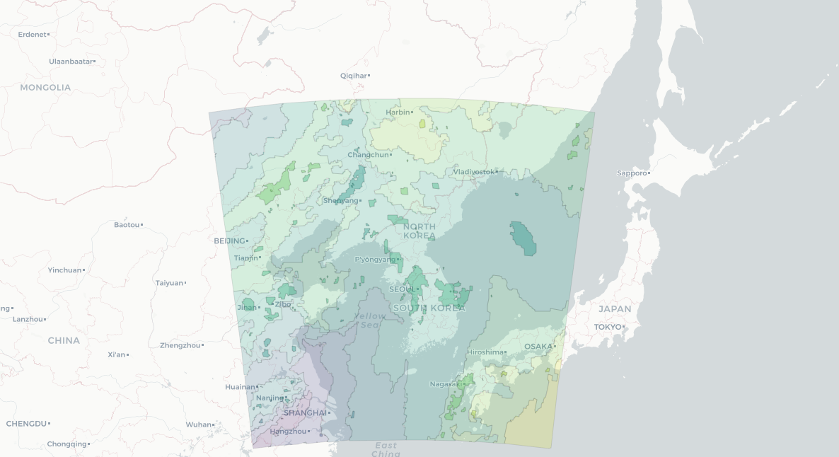
저는 저번에 쓴 위성 자료로 그림을 그려서 한반도 부분만 색칠이 되었습니다.
'대기과학 > 프로그래밍' 카테고리의 다른 글
| [기상청 API][ASOS 시간(hourly) 자료 다운로드] 1. 기본 제공 URL 사용 (0) | 2024.05.24 |
|---|---|
| 관측 자료의 결측을 시각화하기 (0) | 2024.05.22 |
| [folium] 지도에 ASOS 관측소 위치 표시하기 (0) | 2024.05.10 |
| [python] 지도에 대한민국 행정 단위 경계 그리기 (1) | 2024.04.29 |
| 지도에 ASOS 관측소 위치 표시하기 (0) | 2024.04.25 |